Linear Regression

Linear regression is a kind of supervised learning algorithm; you feed some training data to the model, the model learns the best parameters from them and then you use that model to predict some unseen data.

Let us elaborate it a bit. Suppose you have an example dataset of price of houses varying according to the living area; basically a list of tuples of the form: <living area(ft²), price(₹)>. From the context, we know that we want to predict the price of a house given its area. So, area is the independent variable and price is the dependent variable. Remember that you predict the dependent variable's value given the independent variable(s). Now, let us print that example dataset below: 

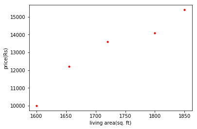
​Let us plot the above dataset:

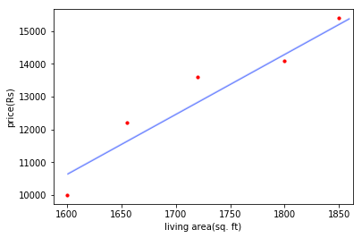
​We can see that as the living area increases, the price is also increasing. The increase is more or less linear(notice 'more or less', not 'strict'). We call such relationship as statistical relationship; the relationship between the dependent and independent variables is not perfect(read not deterministic). Now, we would want to come up with a line that best fits this example set. Something like this maybe:

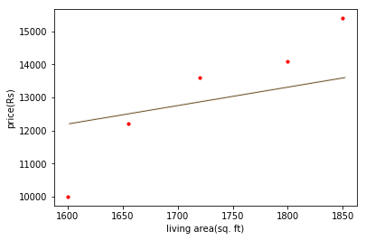
​And not something like this:

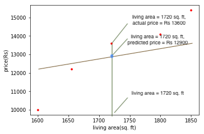
It may be quite intuitive to us that which line among the two is fitting the best. But it is not as trivial to the machine. How do we make the machine understand the notion of 'best fitting line'?By minimizing the error! Let us elaborate a bit on this. For every living area, there is an actual price and a predicted price. The red dot denotes the actual price and the point on the line corresponding to that living area(blue dot on the line) denotes the predicted price.

​We want:

1. The prediction to be as close as to the actual value for every example of living area.
2. ​A single line that minimises this distance between the actual and predicted values.

How can we achieve this? Before moving on, let's revise (and introduce if needed) some terms and variables:

1. ​ Training dataset is a list of tuples of independent and dependent variables: {x⁽ⁱ⁾, y⁽ⁱ⁾}_{i=1 to m}. So, ith example is denoted by (x⁽ⁱ⁾, y⁽ⁱ⁾). Here, x is the independent variable and y is the dependent variable. There are total m examples in this training dataset(hence i = 1 to m​)/
2. Hypotheses h is a linear function of independent variable(s). So, it will be of the form: h_𝜽(x) = 𝞱₁x+𝞱₀. Our aim is to learn the best hypotheses(remember something about 'the best fitting line'? This is it.). It means we have to learn the parameters '𝞱₁' and '𝞱₀' so that the resulting h describes a line that fits the training set the bes​t.
   

So, we want to minimise the error (distance between the actual and predicted values) for every training example. Mathematically, it means to minimise this quantity:

E(𝞱) = 𝚺_{i=1 to m}|y⁽ⁱ⁾-h(x⁽ⁱ⁾)| 

But handling this quantity is mathematically inconvenient (for example, we will need to take derivatives; and we know dealing with the derivative of modulus is avoided if possible). So, we take another quantity which is just the square of the inner terms and call it J(𝞱):

 J(𝞱) = 𝚺_{i=1 to m}(y⁽ⁱ⁾-h(x⁽ⁱ⁾))²

J(𝞱) is called least mean square error.Note that the value of 𝞱 that minimises E(𝞱) would also minimise J(𝞱).Now, it's pretty clear. We obtain the 𝞱 that minimises J(𝞱); this 𝞱 ensures that the error between the actual value and predicted value for all the examples are minimum. Thus, it describes the line that best fits the training dataset. And for predicting, just use the hypotheses h_𝜽; for any new unseen independent variable x_u, the predicted value of the dependent variable will be given by h_𝜽(x_u).But how to minimise J(𝞱)? The answer is Gradient descent. To know how, please have a look here. After running the gradient descent on the training dataset, we obtain the 𝞱 that minimises(approximately) J(𝞱).